x <- 42A Tour of RStudio
Now that you have R and RStudio installed, let’s get familiar with the tool you’ll be using. RStudio is an integrated development environment (IDE) — think of it as the cockpit where you’ll write code, view results, manage files, and explore data, all in one place.
The Four Panes
When you first open RStudio, you’ll see the interface divided into four main panes:
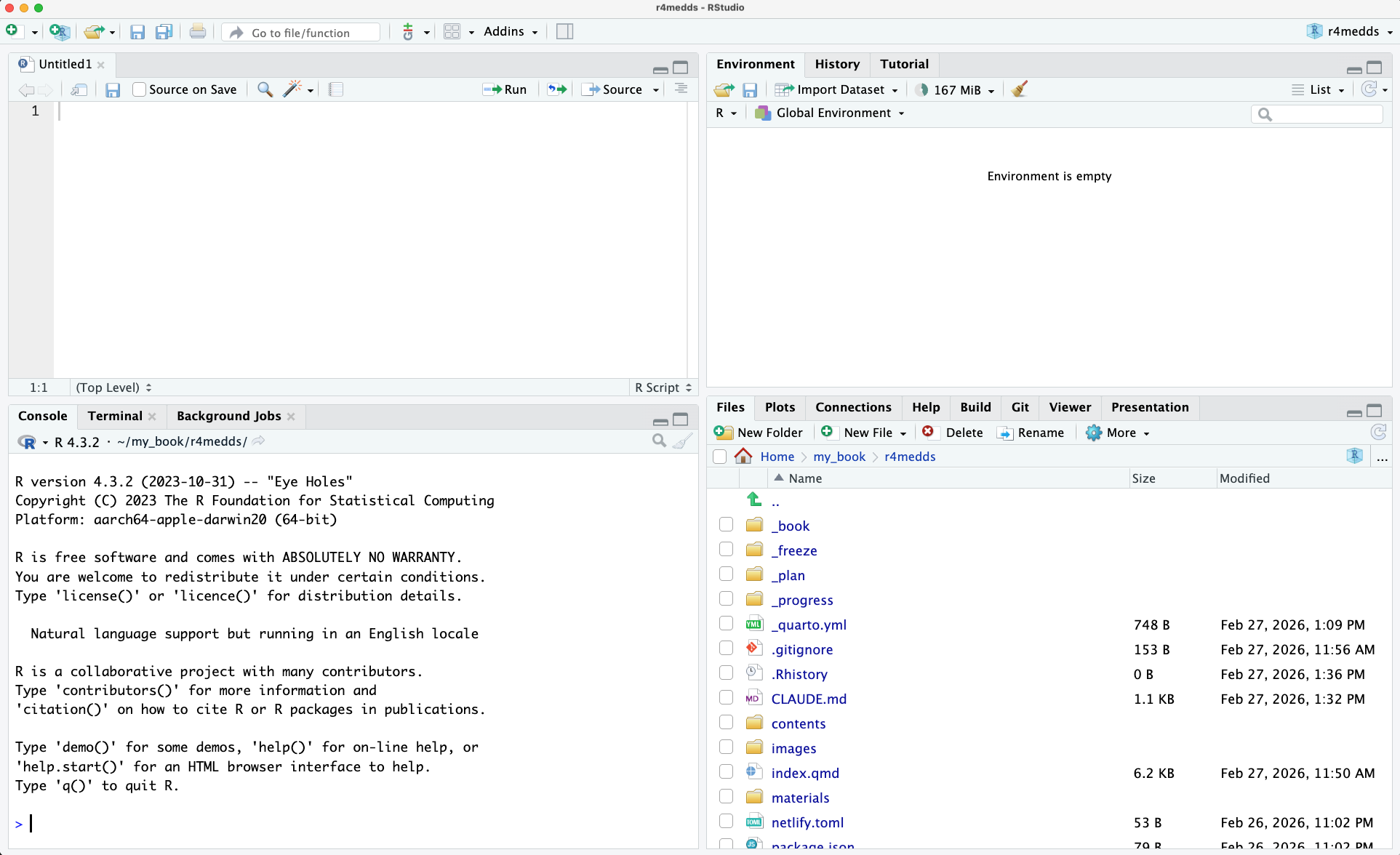
┌───────────────────────┬───────────────────────┐
│                       │                       │
│   1. Source Editor    │   2. Environment      │
│      (top-left)       │      (top-right)      │
│                       │                       │
├───────────────────────┼───────────────────────┤
│                       │                       │
│   3. Console          │   4. Files / Plots /  │
│      (bottom-left)    │      Help / Viewer    │
│                       │      (bottom-right)   │
└───────────────────────┴───────────────────────┘
Let’s walk through each one.
1. Source Editor (top-left)
This is your main workspace — where you write and edit R scripts (.R files), Quarto documents (.qmd files), and other text files. Think of it as your notebook.
Key things to know:
- You can have multiple files open as tabs, just like browser tabs.
- Code you write here is saved to a file — this is how you keep your work reproducible.
- To run a line of code, place your cursor on it and press Cmd + Enter (macOS) or Ctrl + Enter (Windows/Linux).
TipSource vs Console
You can type code directly in the Console, but it won’t be saved. To have a record of things you did, write your code in the Source Editor and run it from there.
2. Environment (top-right)
The Environment pane shows all the objects currently in your R session — variables, data frames, functions, and more. When you create something like:
you’ll see x appear here with a summary of their contents.
This pane also has tabs for:
- History — a log of every command you’ve run in the Console.
- Connections — for connecting to databases (not covered in this book).
- Tutorial — built-in interactive R tutorials from the
learnrpackage.
3. Console (bottom-left)
The Console is where R actually runs your code and displays output. When you press Cmd/Ctrl + Enter in the Source Editor, the code is sent here and executed.
You’ll also see:
- The R startup message when you first open RStudio.
- Output from your code (printed results, messages, warnings).
- Error messages when something goes wrong (we’ll learn how to read these in a later chapter).
The > symbol is the prompt — it means R is ready for your next command.
NoteThe Terminal tab
Next to the Console tab, you’ll notice a Terminal tab. This gives you access to your system’s command-line shell (Bash, Zsh, PowerShell, etc.). We won’t use it much in this book, but it’s useful for tasks like checking quarto --version or running Git commands.
4. Files / Plots / Help (bottom-right)
This is a multi-purpose pane with several important tabs:
- Files — a file browser for your project folder. You can navigate, create, rename, and delete files here.
- Plots — where your graphs appear when you create them with
ggplot2or other plotting functions. - Packages — shows installed R packages and lets you load or install them.
- Help — displays documentation. When you type
?meanin the Console, the help page appears here. - Viewer — for previewing HTML output, Shiny apps, and other interactive content.
TipQuick help lookup
To get help on any R function, type ? followed by the function name in the Console:
?mean
?read_csv
The documentation will appear in the Help tab with a description, arguments, and examples.
File Types in RStudio
When you create a new file in RStudio via File > New File, you’ll see a list of file types:

There are many options, but for this book we only need two: R Script and Quarto Document.
R Script (.R)
An R Script is a plain text file containing only R code. Each line is a command that R can execute. This is the simplest way to write and save your code.
# my_analysis.R
library(tidyverse)

iris |> filter(Sepal.Length > 6) |> summary()
Use R Scripts when you want to write code quickly without any narrative text — for example, a data cleaning pipeline or a utility script.
To create one: File > New File > R Script (or Cmd + Shift + N / Ctrl + Shift + N).
Quarto Document (.qmd)
A Quarto Document lets you combine text and code in the same file — this is called literate programming. Instead of writing code and then separately writing a report about it, you do both in one document. When you render the file, Quarto runs the code and weaves the output (tables, plots, numbers) directly into the final document.
A .qmd file looks like this:
---
title: "Iris Analysis"
format: html
---

## Introduction

This report analyzes the classic iris flower dataset.

```{r}
library(tidyverse)
glimpse(iris)
```

## Results

The mean sepal length is `{r} mean(iris$Sepal.Length)` cm.
This single file produces a complete HTML report with formatted text, code, and output. We’ll explore Quarto in depth in a later chapter.
To create one: File > New File > Quarto Document…
NoteQuarto vs R Markdown — a brief history
If you’ve seen .Rmd files or heard of R Markdown, Quarto is its successor. R Markdown (introduced in 2014) pioneered literate programming in R, and it’s still widely used. Quarto (introduced in 2022) builds on the same ideas but is language-agnostic — it works with R, Python, Julia, and Observable JS.
If you encounter R Markdown files in the wild, don’t worry — the syntax is very similar. For new projects, we recommend Quarto.
Which should I use?
R Script (.R) |
Quarto Document (.qmd) |
|
|---|---|---|
| Contains | Code only | Code + text + output |
| Good for | Quick scripts, utilities, data pipelines | Reports, analyses, presentations |
| Output | None (just runs code) | HTML, PDF, Word, slides |
TipStart with R Scripts
For the first several chapters, we’ll use plain R Scripts to focus on learning R itself. Once you’re comfortable with the language, we’ll switch to Quarto Documents to create reproducible reports.
Running Code in RStudio
There are several ways to run R code. Here are the most common:
| Action | Shortcut |
|---|---|
| Run current line / selection | Cmd + Enter (macOS) / Ctrl + Enter (Windows/Linux) |
| Run entire script | Cmd + Shift + Enter / Ctrl + Shift + Enter |
| Run from beginning to current line | Cmd + Option + B / Ctrl + Alt + B |
Insert code chunk (in .qmd files) |
Cmd + Option + I / Ctrl + Alt + I |
TipThe most important shortcut
If you remember only one shortcut from this book, make it Cmd + Enter (or Ctrl + Enter). You’ll use it hundreds of times.
Create an RStudio Project
Before we start coding, let’s set up an organized workspace. An RStudio Project is a self-contained folder for your work. It automatically sets the working directory, so file paths just work.
- Open RStudio
- Go to File > New Project…
- Select “New Directory”
- Select “New Project”
- Enter a directory name (e.g.,
r4medds-workshop) - Choose where to save it on your computer
- Click “Create Project”
TipWhy use RStudio Projects?
Projects set the working directory automatically. This means read_csv("data/diabetes.csv") will find the file without needing the full path like "/Users/you/Documents/r4medds-workshop/data/diabetes.csv".
It also means you can move the project folder to a different location or share it with someone else, and all the file paths still work.
NoteWhat is a “working directory”?
The working directory is the folder R looks in by default when you read or save files. With an RStudio Project, the working directory is automatically set to the project folder — the one containing the .Rproj file. You can check your current working directory with:
getwd()Customizing RStudio
RStudio is highly customizable. Here are two settings worth exploring early on.
Pane Layout
You can rearrange which tabs appear in which pane. Go to Tools > Global Options > Pane Layout:
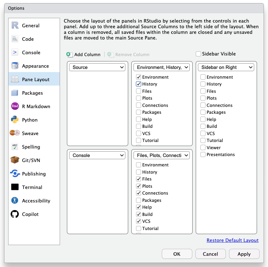
The default layout works well for most people, but you can move things around to suit your workflow. For example, some people prefer having the Console on the top-right instead of the bottom-left.
Appearance
You can change the editor theme, font, and font size. Go to Tools > Global Options > Appearance:
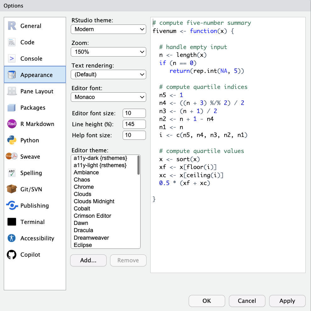
TipTry a dark theme
If you’ll be spending long hours coding, a dark theme (like “Tomorrow Night” or “Dracula”) can reduce eye strain. Pick whatever feels comfortable — you can always change it later.
Summary
You’ve now had a tour of RStudio’s key features:
- The four panes: Source Editor, Console, Environment, and Files/Plots/Help
- How to run code with Cmd/Ctrl + Enter
- How to create an RStudio Project for organized work
- How to customize the layout and appearance
With your environment set up and your way around RStudio, you’re ready to start learning R. Let’s go!